Visualizing the gradient descent method
Por um escritor misterioso
Last updated 26 abril 2025
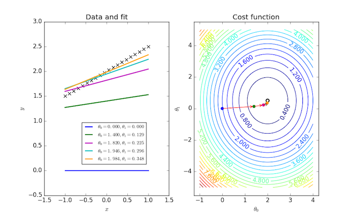
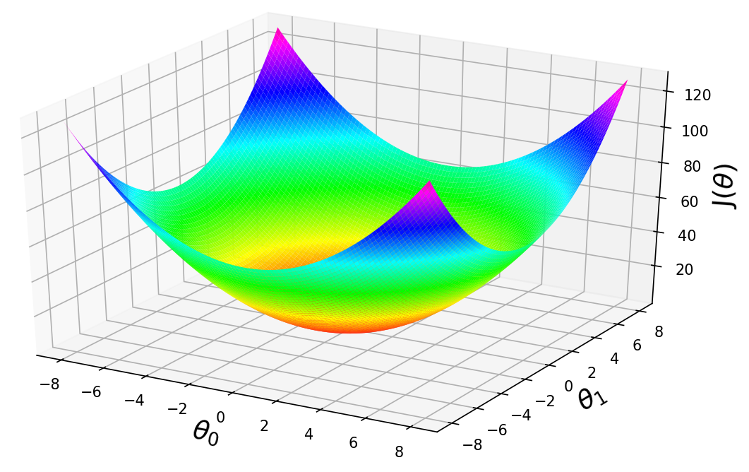
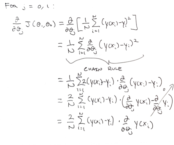
In the gradient descent method of optimization, a hypothesis function, $h_\boldsymbol{\theta}(x)$, is fitted to a data set, $(x^{(i)}, y^{(i)})$ ($i=1,2,\cdots,m$) by minimizing an associated cost function, $J(\boldsymbol{\theta})$ in terms of the parameters $\boldsymbol\theta = \theta_0, \theta_1, \cdots$. The cost function describes how closely the hypothesis fits the data for a given choice of $\boldsymbol \theta$.

How to visualize Gradient Descent using Contour plot in Python
Demystifying Gradient Descent Linear Regression in Python

Simplistic Visualization on How Gradient Descent works
Jack McKew's Blog – 3D Gradient Descent in Python
Gradient Descent With AdaGrad From Scratch
Guide to Gradient Descent Algorithm: A Comprehensive implementation in Python - Machine Learning Space
Visualizing the vanishing gradient problem
Intro to optimization in deep learning: Gradient Descent
Gradient Descent in Machine Learning - Javatpoint
Visualizing the gradient descent in R · Snow of London
Recomendado para você
-
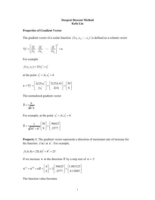
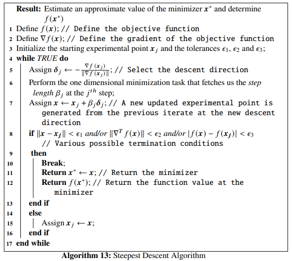
 Steepest Descent Method Search Technique26 abril 2025
 -
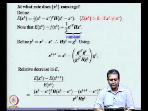 Mod-06 Lec-13 Steepest Descent Method26 abril 2025
 -
 Steepest Descent Method26 abril 2025
 -
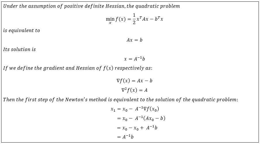 Steepest Descent and Newton's Method in Python, from Scratch: A Comparison, by Nicolo Cosimo Albanese26 abril 2025
 -
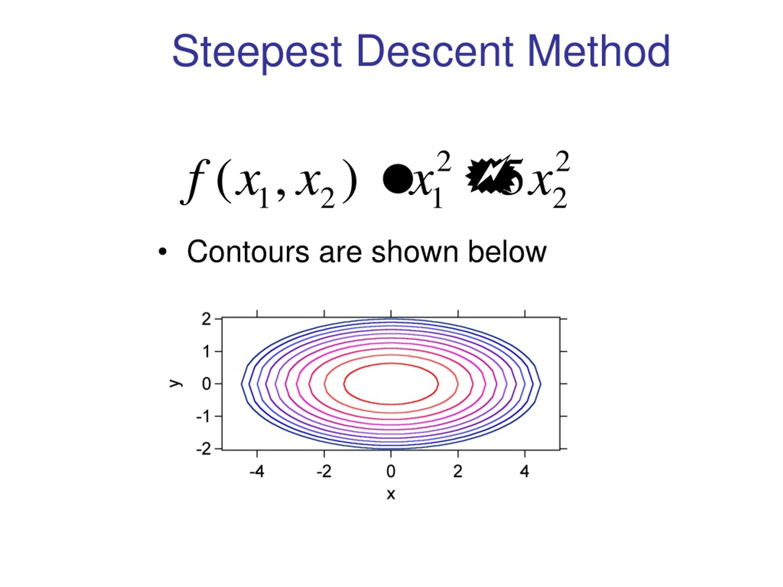 PPT - Steepest Descent Method PowerPoint Presentation, free download - ID:921260526 abril 2025
 -
 Conjugate gradient methods - Cornell University Computational Optimization Open Textbook - Optimization Wiki26 abril 2025
 -
 Chapter 4 Line Search Descent Methods Introduction to Mathematical Optimization26 abril 2025
 -
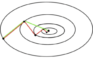
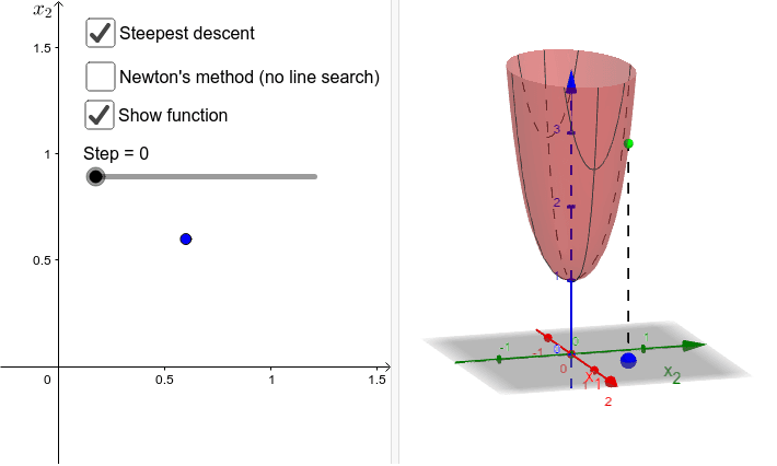 Steepest descent vs gradient method – GeoGebra26 abril 2025
 -
.png) A Beginners Guide to Gradient Descent Algorithm for Data Scientists!26 abril 2025
A Beginners Guide to Gradient Descent Algorithm for Data Scientists!26 abril 2025 -
 Steepest descent method in sc26 abril 2025
você pode gostar
-
 Cheshireeye on X: Eu e a minha mania de gostar de personagem que mal aparece na historia. Sim, to desenhando a candy cat de poppy playtime #PoppyPlaytimeChapter2 #PoppyPlaytime / X26 abril 2025
 -
 The Cuphead Show! The Devil & Ms. Chalice (TV Episode 2022) - IMDb26 abril 2025
 -
PAPA'S WINGERIA - Jogue Grátis Online!26 abril 2025
-
 Kuronuma Suguiyama (@namy_sykes) / X26 abril 2025
 -
 New FIFA 23 Prime Gaming reward pack drops just before TOTS kicks off26 abril 2025
 -
 anime, cute, and pink image Anime sketch, Aesthetic anime, Cute anime profile pictures26 abril 2025
 -
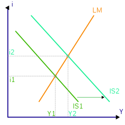 Modelo econômico – Wikipédia, a enciclopédia livre26 abril 2025
 -
 Mumu Fresh “Sometimes Being A Woman” Lyrics Women's Long Sleeve T26 abril 2025
 -
 Elder Scrolls 6 Is Five Years Away? - Gameranx26 abril 2025
 -
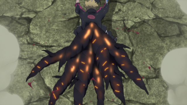 Boruto ep 292 Morte de Boruto e referência a Naruto x Sasuke - Fatos do Mundo Geek26 abril 2025
